

Practice Microsoft Office Specialist: Microsoft Word Expert MO-210 exam. Online Exam Practice Tests with detailed explanations! Pass MO-210 with confidence!
MO-210 - Microsoft Excel (Microsoft 365 Apps) Practice Tests 2026 | Lead1Pass
NEW QUESTION # 13
Instructions
Exam Environment
Exam Interface and Controls
The exam panel provides access to the project task(s). Each project has an associated file in which you will perform the project tasks.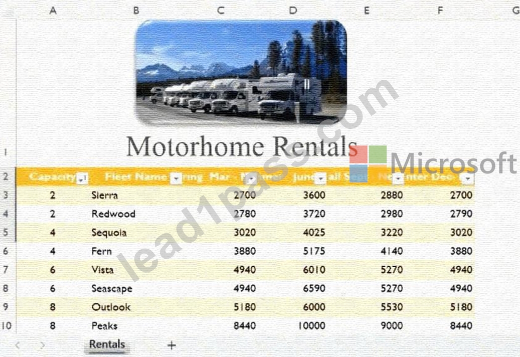
Overview:
Motorhome Rentals
Your company rents motorhomes. The motorhomes rent year-around at different prices. You are preparing pricing worksheets to be shared with others.
Task 3:
Set cells A1:F11 so they will be the only cells that print.
Answer:
Explanation:
See the solution in Explanation below.
Explanation:
To ensure that only a specific range of cells is printed, you need to define aPrint Area. This prevents Excel from printing empty pages or extra data outside of your selection.
Step-by-Step Solution
* Select the range:Use your mouse to click on cellA1and drag your cursor down to cellF11to highlight the entire area.
* Navigate to Page Layout:Click on thePage Layouttab in the top Ribbon.
* Set the Print Area:
* Locate thePage Setupgroup.
* Click on thePrint Areabutton.
* From the drop-down menu, selectSet Print Area.
Once this is set, Excel will only print the content within A1:F11, even if there is data elsewhere on the sheet.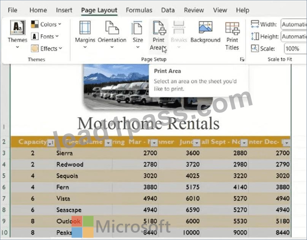
NEW QUESTION # 14
Instructions
Exam Environment
Exam Interface and Controls
The exam panel provides access to the project task(s). Each project has an associated file in which you will perform the project tasks.
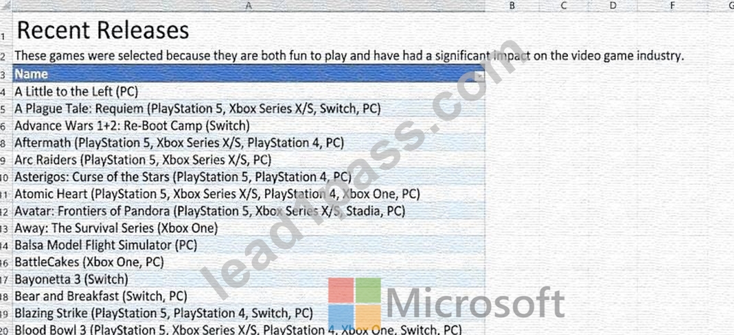
Project 1
Overview:
Video Games
You are tracking video game popularity by compiling a workbook to document your findings.
Task 4:
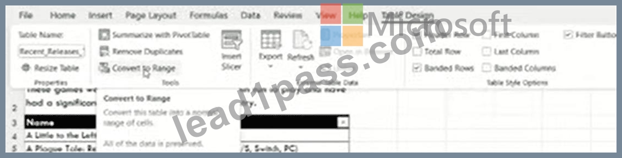
Convert the table on the Recent Releases worksheet to a cell range.
Answer:
Explanation:
Here are the complete solutions below.
Explanation:
Step 1: Select the Table
* Navigate to theRecent Releasesworksheet.
* Clickanywhereinside the data table (for example, click on the text "A Little to the Left").
* Note:You do not need to highlight the whole table; just clicking one cell inside it is enough to activate the hidden menu.
Step 2: Go to the "Table Design" Tab
* Look at the Ribbon at the very top of the Excel window.
* Because you clicked inside the table, a new tab calledTable Design(or sometimes justDesign) will appear on the far right side of the Ribbon.
* Click on theTable Designtab.
Step 3: Click "Convert to Range"
* In theTable Designtoolbar, look for theToolsgroup (usually on the left side).
* Click the button labeledConvert to Range.
Visual Reference:
Step 4: Confirm the Action
* A confirmation dialog box will pop up asking:"Do you want to convert the table to a normal range?"
* ClickYes.
Result:The table functionality (like the little filter arrows next to the headers) will disappear, but the cell colors and data will remain exactly where they are. The data is now a standard "Range."
NEW QUESTION # 15
Instructions
Exam Environment
Exam Interface and Controls
The exam panel provides access to the project task(s). Each project has an associated file in which you will perform the project tasks.
Overview:
Motorhome Rentals
Your company rents motorhomes. The motorhomes rent year-around at different prices. You are preparing pricing worksheets to be shared with others.
Task5:
On the Rentals worksheet, configure the heading row in the table so that entries wider than the column wrap to multiple lines.
Answer:
Explanation:
See the solution in Explanation below.
Explanation:
To ensure that the text in your heading row (the table headers) is fully visible without changing the column width, you will use theWrap Textfeature.
Step-by-Step Solution
* Select the Header Row:In your "Rentals" worksheet, click and drag to select the cell rangeA2:F2(the orange heading row containing "Capacity," "Fleet Name," etc.).
* Navigate to the Home Tab:Ensure you are on theHometab of the Ribbon.
* Apply Wrap Text:
* Look for theAlignmentgroup.
* Click theWrap Textbutton (usually represented by an "ab" icon with a curved arrow).
* Verify the Result:The text in your headers will now automatically wrap to multiple lines if it exceeds the current width of the column.
NEW QUESTION # 16
Instructions
Exam Environment
Exam Interface and Controls
The exam panel provides access to the project task(s). Each project has an associated file in which you will perform the project tasks.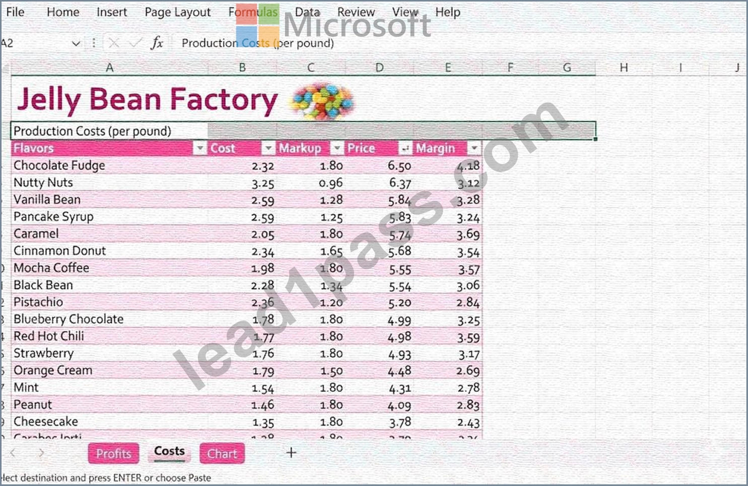
Overview:
Jelly Beans
A shop you manage sells gourmet jelly beans. You are tracking the amount of jelly beans sold each quarter and summarizing the information in aworkbook.
Task 5:
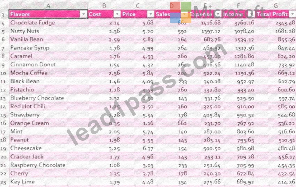
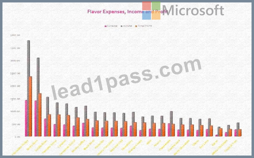
Group the Profits, Costs, and Chart worksheets and change the tab color to Pink, Accent 4.
Answer:
Explanation:
See the solution in Explanation below.
Explanation:
To group multiple worksheets and change their tab colors simultaneously in Microsoft Excel 365, follow these steps:
Step 1: Group the Worksheets
* Look at the worksheet tabs at the bottom of your Excel window.
* Click on the first tab,Profits.
* Hold down theCtrlkey on your keyboard.
* While holdingCtrl, click on theCoststab and then theCharttab.
* Note: You will notice all three tabs now have a white background, indicating they are grouped together.
Step 2: Change the Tab Color
* Right-clickon any of the selected (grouped) tabs.
* Hover your mouse overTab Colorin the pop-up menu.
* In the color palette that appears, locate theTheme Colorssection.
* Find and selectPink, Accent 4(this is usually the 8th color in the top row of the Theme Colors section).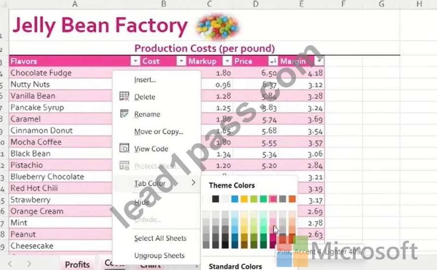
Step 3: Ungroup the Worksheets
* To finish,right-clickon any of the tabs again.
* SelectUngroup Sheetsfrom the menu.
* Alternatively, you can click on any worksheet tab that is not part of the group to ungroup them.
Final Result
TheProfits,Costs, andCharttabs will now all display the samePink, Accent 4color at the bottom of your workbook.
Would you like me to help you with the next task or another project?
NEW QUESTION # 17
Instructions
Exam Environment
Exam Interface and Controls
The exam panel provides access to the project task(s). Each project has an associated file in which you will perform the project tasks.
Overview:
Jelly Beans
A shop you manage sells gourmet jelly beans. You are tracking the amount of jelly beans sold each quarter and summarizing the information in aworkbook.
Task 4:
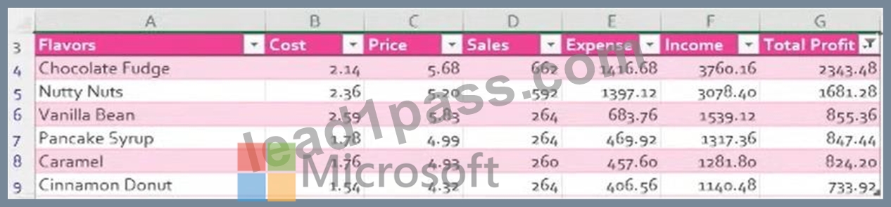
Filter the Profits worksheet to display only flavors with Total Profit that are Above Average.
Answer:
Explanation:
See the solution in Explanation below.
Explanation:
To filter theProfitsworksheet to display only the flavors with aTotal Profitthat isAbove Average, follow these steps:
Step 1: Access the Profits Worksheet
* Click on theProfitsworksheet tab at the bottom of the Excel window.
Step 2: Apply the Above Average Filter
* Look at theTotal Profitheader (CellG3). If you don't see a small drop-down arrow next to it, go to the Datatab and clickFilter.
* Click theFilter Drop-down Arrowin theTotal Profitheader cell.
* Hover your mouse overNumber Filtersin the menu that appears.
* From the side menu, selectAbove Average.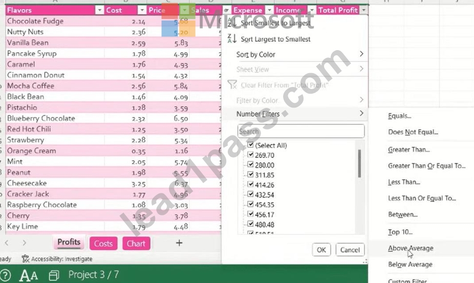
Step 3: Verify the Results
* Excel will automatically calculate the average of all values in the "Total Profit" column and hide any rows that fall below that number.
* You will notice the row numbers on the left are now blue, indicating a filter is active.
NEW QUESTION # 18
Instructions
Exam Environment
Exam Interface and Controls
The exam panel provides access to the project task(s). Each project has an associated file in which you will perform the project tasks.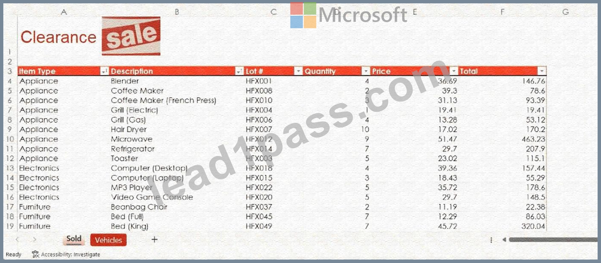
Overview:
Clearance Sale
You are the administrative assistant for a retail company that is going out of business. You've been tasked to prepare a workbook for the clearance sale.
Task5:
On the Vehicles worksheet, in the Code column cell B4, create a formula that returns the two leftmost letters of the vehicle style displayed in cell D4.
Answer:
Explanation:
See the solution in Explanation below.
Explanation:
To extract specific characters from the start of a text string in Excel, you use theLEFTfunction.
Step-by-Step Solution
* Navigate to the Worksheet: Click on theVehiclesworksheet tab at the bottom of your Excel window.
* Select Cell B4: Click on cellB4(under the "Code" column).
* Enter the Formula: Type the following formula exactly as shown: =LEFT(D4, 2)
* Press Enter: Once you press Enter, Excel will look at the "Vehicle Style" in cellD4and return only the firsttwoletters.
Explanation of the Formula
* LEFT: This is the function used to start counting characters from the beginning (left side) of a cell.
* D4: This tells Excel which cell contains the text you want to extract from (the Vehicle Style).
* 2: This specifies the number of characters you want to retrieve.
NEW QUESTION # 19
Instructions
Exam Environment
Exam Interface and Controls
The exam panel provides access to the project task(s). Each project has an associated file in which you will perform the project tasks.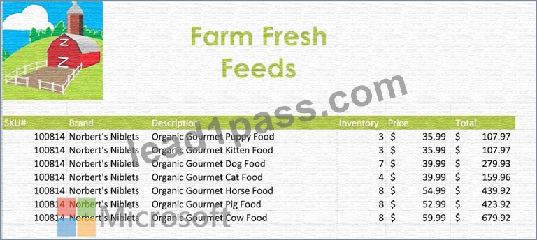
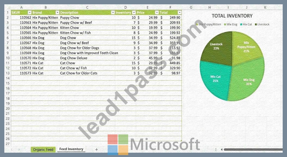
Farm Feeds:
You are the assistant manager for a farm pet feed store. You are creating an inventory report.
Task 4:
On the Organic Feed worksheet, format the data range A3:F10 as a table that has headers. Apply the Lime, Table Style Light 14 format.
Answer:
Explanation:
See the solution in Explanation below.
Explanation:
To completeTask 4: Format a range as a table with a specific style on the Organic Feed worksheet, follow these steps:
Step 1: Select the "Organic Feed" Worksheet
Navigate to the correct worksheet by clicking theOrganic Feedtab at the bottom of the Excel window.
Step 2: Select the Data Range
Highlight the specific range mentioned in the task:
* Click and drag your mouse to select cells fromA3toF10.
* Ensure the selection includes the header row (SKU#, Brand, Description, etc.) and all data rows down to row 10.
Step 3: Format as Table
* Go to theHometab on the Ribbon.
* In theStylesgroup, click theFormat as Tablebutton.
Step 4: Apply the Specific Table Style
* A gallery of styles will appear. Look for theLightsection.
* Find and click onLime, Table Style Light 14(this is usually the last style in the second row of the Light section, featuring a lime green header).
Step 5: Confirm Headers
* A small "Format As Table" dialog box will pop up.
* Ensure the checkbox forMy table has headersischecked.
* ClickOK.
Final Result
The data range will now be converted into a functional table with filter buttons in the header row and the lime green styling applied.
NEW QUESTION # 20
Instructions
Exam Environment
Exam Interface and Controls
The exam panel provides access to the project task(s). Each project has an associated file in which you will perform the project tasks.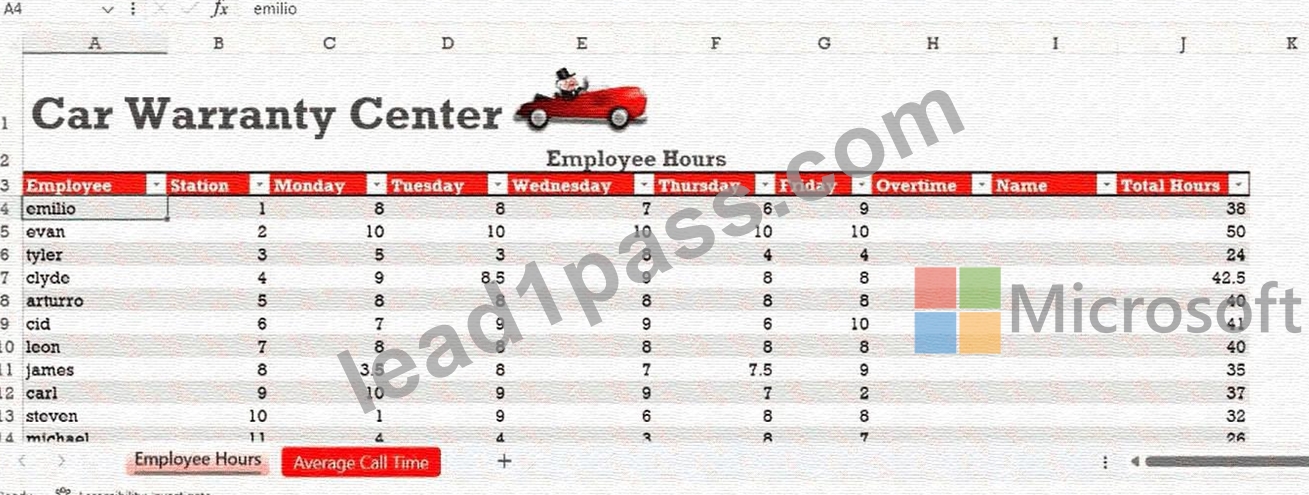
Overview:
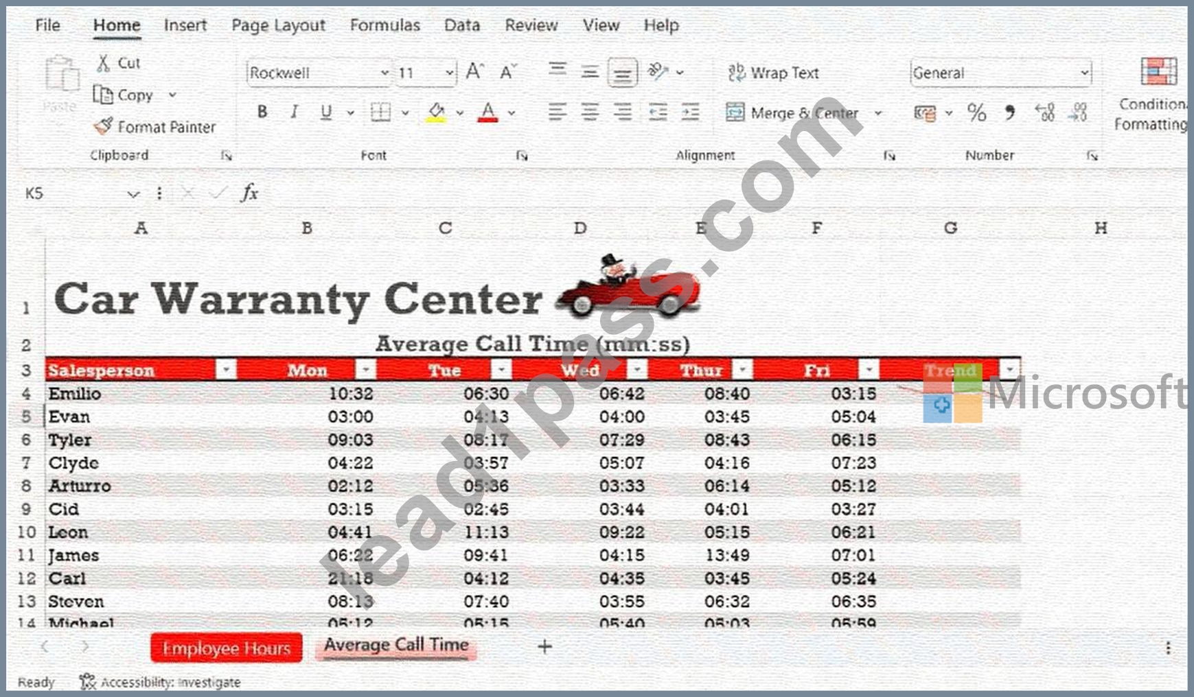
Car Warranty
You are the supervisor for a Car Warranty Center. You use Excel to report employee hours and telephone calls.
Task5:
On the Average Call Time worksheet, create a 3-D Clustered Column chart that shows the call times for each Salesperson from Mon through Fri. Insertthe Chart Title Average Call Time. Position the new chart below the table.
Answer:
Explanation:
See the solution in Explanation below.
Explanation:
To completeTask 5, you will create a 3-D Clustered Column chart on theAverage Call Timeworksheet to visualize the weekly performance of each salesperson.
Step 1: Navigate to the Worksheet
Click on theAverage Call Timetab at the bottom of your Excel window to switch views.
Step 2: Select the Data Range
You need to select the names and the call times for all five days (Monday through Friday), butexcludethe
"Trend" column:
* Click and drag to select cellsA3 to F14.
* Note:This includes the header row (Salesperson, Mon, Tue, etc.) and all employee rows down to Michael.
Step 3: Insert the 3-D Clustered Column Chart
* Go to theInserttab on the Ribbon.
* In theChartsgroup, click theInsert Column or Bar Charticon (it looks like small vertical bars).
* Under the3-D Columnsection, select the first option:3-D Clustered Column.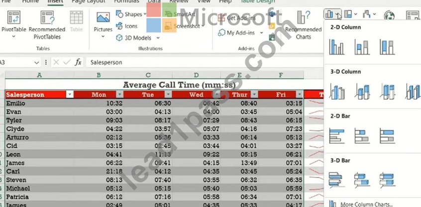
Step 4: Add the Chart Title
* Click once on the default text that says "Chart Title" at the top of the new chart.
* TypeAverage Call Timeand pressEnter(or click outside the text box).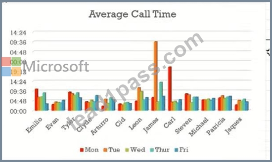
Step 5: Position the Chart
* Hover your mouse over a blank area of the chart (the chart area).
* Click and drag the chart so it is positionedbelow the table.
* Placement Tip:Usually, starting the chart around row 17 or 18 is ideal so it doesn't overlap your data.
NEW QUESTION # 21
Instructions
Exam Environment
Exam Interface and Controls
The exam panel provides access to the project task(s). Each project has an associated file in which you will perform the project tasks.
Farm Feeds:
You are the assistant manager for a farm pet feed store. You are creating an inventory report.
Task 5:
On the Feed Inventory worksheet, apply Style 5 to the chart.
Answer:
Explanation:
See the solution in Explanation below.
Explanation:
To completeTask 5: Apply Style 5 to the chart on the Feed Inventory worksheet, follow these exact steps:
Step 1: Select the "Feed Inventory" Worksheet
Ensure you are on the correct sheet by clicking theFeed Inventorytab at the bottom of your Excel window.
Step 2: Select the Chart
Click anywhere on theTotal Inventorypie chart to select it. When selected, you will see a border around the chart and new tabs will appear on the Ribbon.
Step 3: Open Chart Design Tools
With the chart selected, look at the top Ribbon and click on theChart Designtab (this tab only appears when a chart is active).
Step 4: Apply Chart Style 5
* In theChart Stylesgroup, you will see a gallery of different looks for your chart.
* Hover your mouse over the styles to see their names, or click theMorearrow (the small downward arrow at the bottom right of the styles gallery) to see all options.
* Locate and click onStyle 5.
Note:Style 5 typically features a specific layout of data labels and a distinct background or border style that matches the "Farm Fresh Feeds" theme.
Final Result
The pie chart will update its appearance to match Style 5, adjusting the placement of the percentage labels and the overall color shading to remain consistent with your report's professional look.
NEW QUESTION # 22
Instructions
Exam Environment
Exam Interface and Controls
The exam panel provides access to the project task(s). Each project has an associated file in which you will perform the project tasks.
Overview:
Jelly Beans
A shop you manage sells gourmet jelly beans. You are tracking the amount of jelly beans sold each quarter and summarizing the information in aworkbook.
Task 2:
Use a builtin Excel feature to copy all of the formatting of cell range A2:G2 located on the Profits worksheet and apply that formatting to cell A2 on theCosts worksheet.
Answer:
Explanation:
See the solution in Explanation below.
Explanation:
To transfer the formatting from theProfitsworksheet to theCostsworksheet while maintaining consistency, follow these steps:
Step 1: Copy the Source Formatting
* Click on theProfitsworksheet tab at the bottom of your Excel window.
* Select the cell rangeA2:G2.
* On theHometab, in theClipboardgroup, click theFormat Painterbutton (it looks like a paintbrush).
* Tip: Your cursor will now have a small paintbrush icon next to it, indicating the formatting is
"loaded" and ready to be pasted.
Step 2: Apply Formatting to the Destination
* Click on theCostsworksheet tab (the one shown in your provided image).
* Click directly onCell A2(the cell containing "Production Costs (per pound)").
* Excel will automatically apply the formatting across the range starting from A2 to match the original source.
Final Result
The cell range in theCostsworksheet should now match the style (font, background color, and borders) of the Profitsworksheet. The grey shading currently visible in your image in rangeB2:G2will be replaced by the style from the first sheet.
NEW QUESTION # 23
Instructions
Exam Environment
Exam Interface and Controls
The exam panel provides access to the project task(s). Each project has an associated file in which you will perform the project tasks.
Overview:
Clearance Sale
You are the administrative assistant for a retail company that is going out of business. You've been tasked to prepare a workbook for the clearance sale.
Task 3:
Configure the Sold worksheet so rows 1 through 3 remain visible as you scroll vertically.
Answer:
Explanation:
See the solution in Explanation below.
Explanation:
To keep rows 1 through 3 visible while you scroll down the "Sold" worksheet, you will use theFreeze Panes feature.
Step-by-Step Solution
* Select Row 4: Click on the row number4on the far left of the screen to select the entire row.
* Note: In Excel, "Freeze Panes" freezes everythingabovethe currently selected row.
* Navigate to the View Tab: Click on theViewtab in the top Ribbon menu.
* Click Freeze Panes: In theWindowgroup, click theFreeze Panesbutton.
* Select Freeze Panes: From the drop-down menu, select the first option,Freeze Panes.
Verification
Scroll down the worksheet using your mouse or the scroll bar. You should notice that the "Clearance Sale" header and the "Item Type/Description/etc." header row (rows 1-3) stay locked at the top of the screen while the data in row 4 and below moves.
NEW QUESTION # 24
Instructions
Exam Environment
Exam Interface and Controls
The exam panel provides access to the project task(s). Each project has an associated file in which you will perform the project tasks.
Project 1
Overview:
Video Games
You are tracking video game popularity by compiling a workbook to document your findings.
Task 2:
On the Top 20 Videos worksheet, change the width of column C to 2.
Answer:
Explanation:
Here are the complete solutions below.
Explanation:
Step-by-Step Instructions
* Navigate to the Correct Worksheet:
* Click on the tab labeled Top 20 Videos at the bottom of the Excel window to ensure you are on the correct sheet.
* Select Column C:
* Click on the letter C in the column header to select the entire column.
* Open Column Width Settings:
* Method A (Ribbon): Go to the Home tab. In the Cells group (towards the right), click Format.
Select Column Width... from the dropdown menu.
* Method B (Right-click): Right-click directly on the column header "C". A context menu will appear. Click Column Width...
* Enter the Width:
* A small dialog box labeled "Column Width" will appear.
* Type 2 in the box.
* Click OK.
Visual Verification
Before: Column C (containing the "Year" data) is likely wider, fitting the four-digit years comfortably.
After: Column C will become very narrow. The "Year" header and the dates (like 2011, 1984) might display as hashes (####) because the column is now too narrow to display the numbers, or the text will simply be cut off. This is expected behavior for the exam task; do not widen it back out unless instructed to do so.
NEW QUESTION # 25
Instructions
Exam Environment
Exam Interface and Controls
The exam panel provides access to the project task(s). Each project has an associated file in which you will perform the project tasks.
Farm Feeds:
You are the assistant manager for a farm pet feed store. You are creating an inventory report.
Task 2:
Import NewFeeds.txt located in the GMetrixTemplates folder as a table on a new worksheet.
Answer:
Explanation:
See the solution in Explanation below.
Explanation:
To completeTask 2: Import NewFeeds.txt as a table on a new worksheet, follow these exact steps in Microsoft Excel 365:
Step 1: Open the Import Tool
* Go to theDatatab on the top Ribbon.
* In theGet & Transform Datagroup, click onFrom Text/CSV.
Step 2: Locate the File
* A file browser window will open. Navigate to theGMetrixTemplatesfolder.
* Select the file namedNewFeeds.txt.
* ClickImport.
Step 3: Configure the Import Preview
* A preview window will appear. Excel should automatically detect the delimiter (usually a tab or comma).
* Ensure theFile OriginandDelimiterlook correct in the preview.
* Instead of clicking "Load," click thearrow next to the Load buttonand selectLoad To....
Step 4: Import as a Table on a New Worksheet
* In theImport Datadialog box that appears, select the radio button forTable.
* Under "Where do you want to put the data?", selectNew worksheet.
* ClickOK.
Final Result
Excel will create a brand new sheet (e.g., "Sheet2") and place the contents of NewFeeds.txt inside a formatted Excel Table.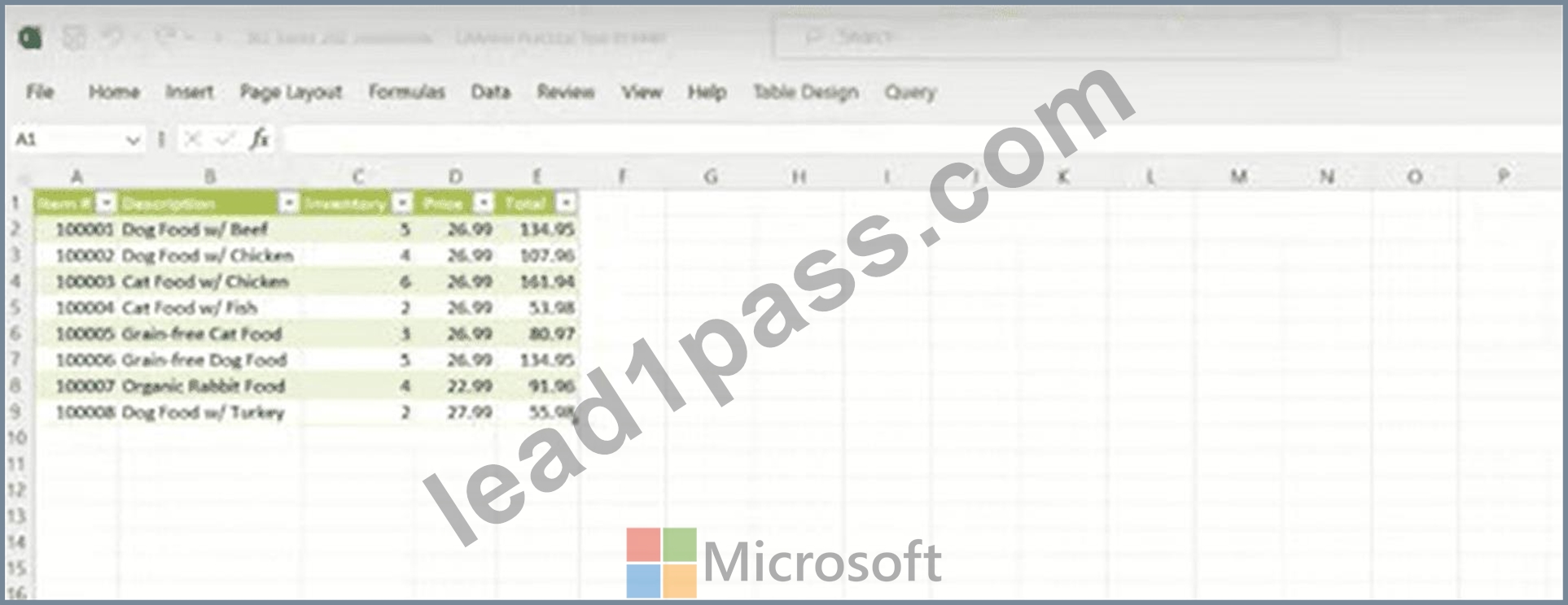
NEW QUESTION # 26
Instructions
Exam Environment
Exam Interface and Controls
The exam panel provides access to the project task(s). Each project has an associated file in which you will perform the project tasks.
Overview:
Motorhome Rentals
Your company rents motorhomes. The motorhomes rent year-around at different prices. You are preparing pricing worksheets to be shared with others.
Task 2:
Add the value New Rates to the Title property of the document.
Answer:
Explanation:
See the solution in Explanation below.
Explanation:
To add a value to theTitleproperty of an Excel document, you need to access the Backstage view. This metadata is helpful for organizing and searching for files.
Step-by-Step Solution
* Click on theFiletab in the top-left corner of the Excel ribbon.
* Ensure thatInfois selected in the left-hand sidebar.
* On the right side of the screen, you will see a section labeledProperties.
* Locate the field namedTitle. If it says "Add a title," click directly on that text.
* TypeNew Ratesinto the text box.
* Click anywhere else on the screen or pressEnterto save the property.
* Click theBack arrowin the top-left corner to return to your worksheet.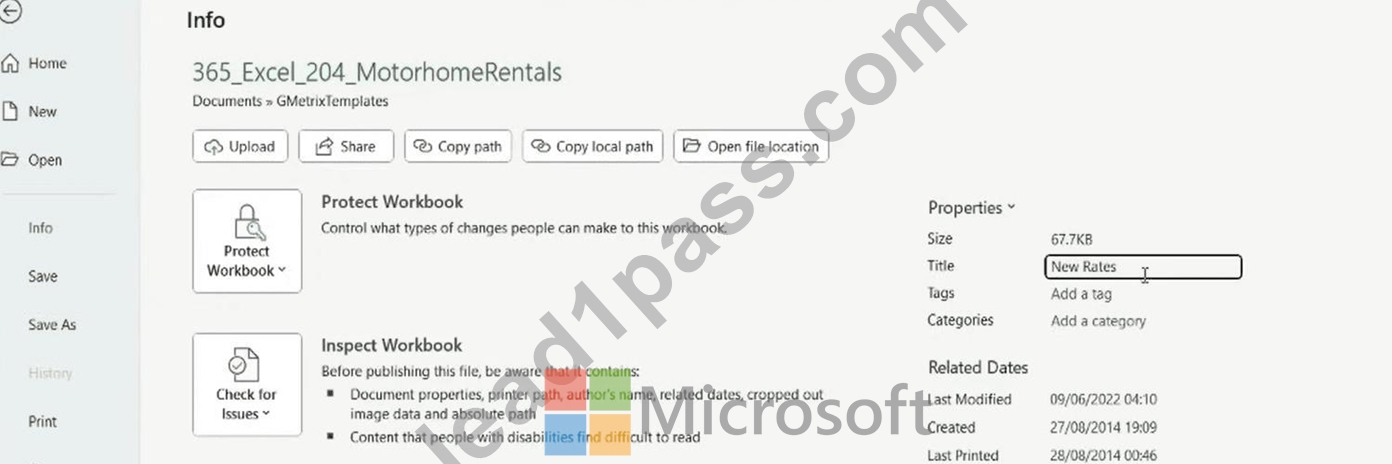
NEW QUESTION # 27
......
Get instant access to MO-210 practice exam questions: https://drive.google.com/open?id=19EvTuZuDkweAh08EjexHFZldu-rPRPTB
The best MO-210 exam study material and preparation tool is here: https://www.lead1pass.com/Microsoft/MO-210-practice-exam-dumps.html